We have examined some of the basic questions in time-series analysis, specifically are there clear trends in our data over time, and does there appear to be a seasonal influence in the data?
However, there are some key aspects of time-series data that are important to explore before we begin to undertake any statistical analysis of the data.
Registered S3 method overwritten by 'quantmod':
  method            from
  as.zoo.data.frame zoo
library(ggplot2)library(tseries)# Function to generate a stationary time seriesgenerate_stationary_ts <-function(n) {# AR(1) process with a coefficient that ensures stationarity (absolute value < 1)arima.sim(model =list(ar =0.5), n = n)}# Generate time series datastationary_ts <-generate_stationary_ts(120)rm(generate_stationary_ts)
Prepare the dataset
Now, I’m going to prepare that data for analysis. Notice that I have ‘told’ R that the data is in monthly format (12 observations per year) and that the start date is January 2023.
Rather than create a new object, I have simply replaced the existing dataframe stationary_ts with a time-series object of the same name.
# Convert to ts objectstationary_ts <-ts(stationary_ts, frequency =12, start =c(2010, 1)) # This includes data starts from Jan 2010
Visual inspection
Show code
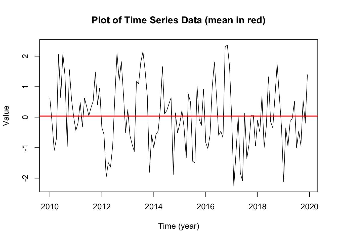
# Plot the generated time series dataplot(stationary_ts, main ="Plot of Time Series Data (mean in red)", xlab ="Time (year)", ylab ="Value")# add the mean value# Calculate mean of the time seriesmean_value <-mean(stationary_ts, na.rm =TRUE) # na.rm = TRUE ensures NA values are ignored# Add a horizontal line at the mean valueabline(h = mean_value, col ="red", lwd =2) # 'h' spe
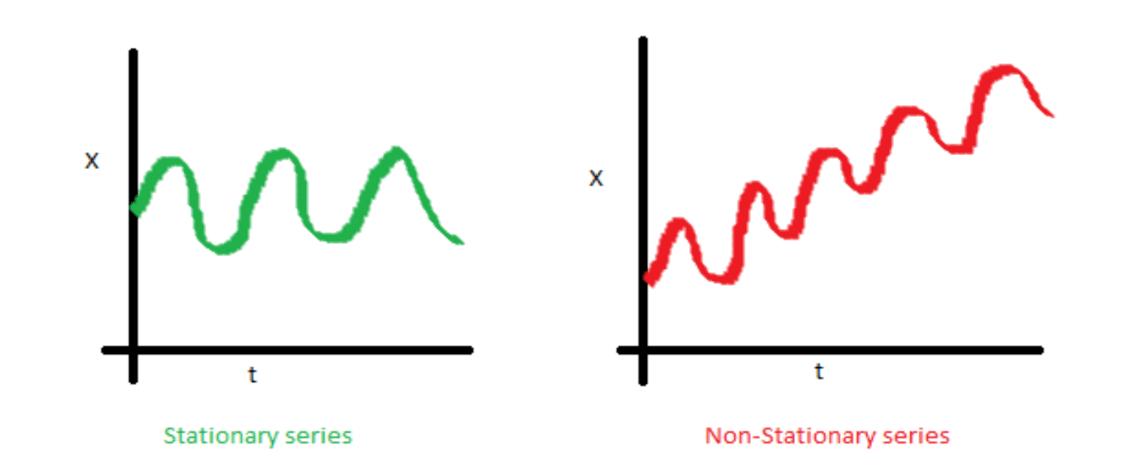
Note that the plotted figure shows no clear trends. It seems to ‘hover’ around the mean. This suggests that the data is stationary.
Testing for stationarity
The Augmented Dickey-Fuller (ADF) test is often used to test for stationarity. It tests the null hypothesis that a unit root is present in a time series sample.
library(urca)# Perform the Augmented Dickey-Fuller Testadf_test <-ur.df(stationary_ts, type ="drift", lags =1)# View the summary of the test, including critical valuessummary(adf_test)
###############################################
# Augmented Dickey-Fuller Test Unit Root Test #
###############################################

Test regression drift


Call:
lm(formula = z.diff ~ z.lag.1 + 1 + z.diff.lag)

Residuals:
     Min       1Q   Median       3Q      Max
-2.17411 -0.65466 -0.04125  0.69066  2.52076

Coefficients:
            Estimate Std. Error t value Pr(>|t|)
(Intercept)  0.02649    0.09238   0.287    0.775
z.lag.1     -0.66179    0.10430  -6.345 4.54e-09 ***
z.diff.lag   0.06826    0.09370   0.728    0.468
---
Signif. codes:  0 '***' 0.001 '**' 0.01 '*' 0.05 '.' 0.1 ' ' 1

Residual standard error: 1.003 on 115 degrees of freedom
Multiple R-squared:  0.3096,    Adjusted R-squared:  0.2976
F-statistic: 25.79 on 2 and 115 DF,  p-value: 5.6e-10


Value of test-statistic is: -6.3453 20.1393

Critical values for test statistics:
      1pct  5pct 10pct
tau2 -3.46 -2.88 -2.57
phi1  6.52  4.63  3.81
What does this output tell us?
If the test statistic is less (more negative) than the critical value at a certain significance level (e.g., -3.45 < -2.86 at the 5% level), and/or if the p-value is small (typically < 0.05), you can reject the null hypothesis. This suggests that the time series is stationary.
If the test statistic is greater (less negative) than the critical value at the chosen significance level (e.g., -2.50 > -2.86 at the 5% level), and/or if the p-value is large (typically > 0.05), you cannot reject the null hypothesis. This suggests that the time series is non-stationary.
In the case above, the test statistic (-5.6412) is less than the critical value at 5% level (-2.88) and the p-value is < 0.01. We can reject the null hypothesis, and conclude that our data is stationary.
52.3 Examining stationarity 2: demonstration
Create a synthetic dataset
I’m going to create another synthetic dataset that has a clear trend (and in-built seasonality).
Show code to create synthetic dataset
rm(list=ls())# Load necessary librarylibrary(forecast)# Set seed for reproducibilityset.seed(1234)# Generate Time Series Data# Creating a time series with trend and seasonalitytime_points <-120# e.g., 120 months (10 years of monthly data)trend_component <-seq(1, time_points, by =1)seasonal_component <-sin(seq(1, time_points, by =1) *2* pi /12) *5random_noise <-rnorm(time_points, mean =0, sd =2)# Combine components to create final time series datats_data <- trend_component + seasonal_component + random_noiserm(random_noise, seasonal_component, time_points, trend_component)
Prepare the dataset
Now, I’m going to prepare that data for analysis
# Convert to ts objectts_data <-ts(ts_data, frequency =12, start =c(2010, 1)) # This includes data starts from Jan 2010
Visual inspection
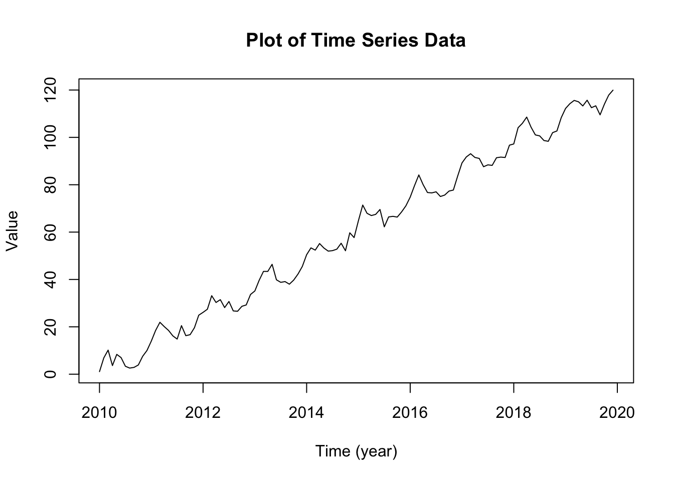
# Plot time series dataplot(ts_data, main ="Plot of Time Series Data", xlab ="Time (year)", ylab ="Value")
Note that the plotted figure shows a clear upwardtrend in the data over time. Also, note that the data seems to rise, fall, rise more, fall and on on.
The appearance of a trend in our data raises suspicions that the data is non-stationary.
Testing for stationarity
Visual inspection is always useful, but statistical tests are usually preferable.
As you know, the Augmented Dickey-Fuller (ADF) test is commonly used to test for stationarity. It tests the null hypothesis that a unit root is present in a time series sample.
Show code
library(urca)# Perform the Augmented Dickey-Fuller Testadf_test <-ur.df(ts_data, type ="drift", lags =1)# View the summary of the test, including critical valuessummary(adf_test)
###############################################
# Augmented Dickey-Fuller Test Unit Root Test #
###############################################

Test regression drift


Call:
lm(formula = z.diff ~ z.lag.1 + 1 + z.diff.lag)

Residuals:
   Min     1Q Median     3Q    Max
-8.277 -2.077 -0.078  2.209  6.635

Coefficients:
             Estimate Std. Error t value Pr(>|t|)
(Intercept)  1.065902   0.587177   1.815   0.0721 .
z.lag.1     -0.001868   0.008417  -0.222   0.8247
z.diff.lag   0.004755   0.092427   0.051   0.9591
---
Signif. codes:  0 '***' 0.001 '**' 0.01 '*' 0.05 '.' 0.1 ' ' 1

Residual standard error: 3.143 on 115 degrees of freedom
Multiple R-squared:  0.0004434, Adjusted R-squared:  -0.01694
F-statistic: 0.02551 on 2 and 115 DF,  p-value: 0.9748


Value of test-statistic is: -0.2219 4.9703

Critical values for test statistics:
      1pct  5pct 10pct
tau2 -3.46 -2.88 -2.57
phi1  6.52  4.63  3.81
What does this output tell us?
If the test statistic is less (more negative) than the critical value at a certain significance level (e.g., -3.45 < -2.86 at the 5% level), and/or if the p-value is small (typically < 0.05), you can reject the null hypothesis. This suggests that the time series is stationary.
If the test statistic is greater (less negative) than the critical value at the chosen significance level (e.g., -2.50 > -2.86 at the 5% level), and/or if the p-value is large (typically > 0.05), you cannot reject the null hypothesis. This suggests that the time series is non-stationary.
In the case above, the test statistic (-0.2219) is greater than the critical value at 5% level (-2.88) and the p-value is >0.05. We cannot reject the null hypothesis, and therefore must conclude that our data is non-stationary. This confirms what we suspected based on visual inspection.
52.4 Differencing the time series: demonstration
So we have a problem with this second data set. It is non-stationary. We can’t proceed with further statistical analysis of time-series data until this is addressed!
Differencing is a method of transforming a non-stationary time series into a stationary one. This is done by subtracting the previous observation from the current observation.
Differencing can help stabilise the mean of a time series by removing changes in the level of a time series, thus eliminating (or reducing) trend and seasonality.
First differencing
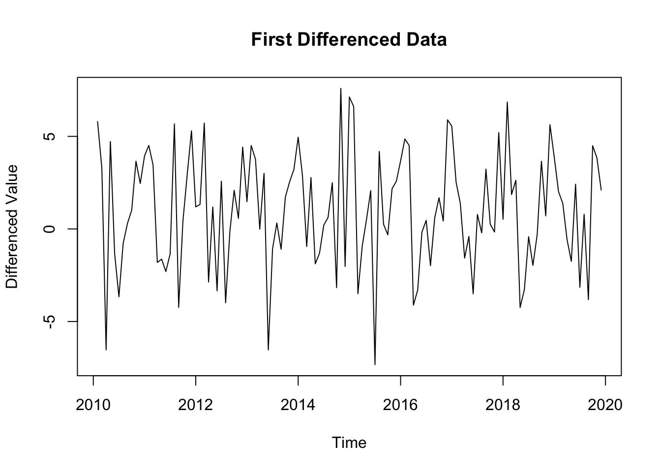
By applying first-order differencing to the object ts_data, we achieve a visual pattern that suggests stationarity in the data.
diff_ts_data <-diff(ts_data, differences =1) # create new object with differencing# Plot the differenced dataplot(diff_ts_data, main="First Differenced Data", xlab="Time", ylab="Differenced Value")
Visually, this looks more like what we would expect if our data was stationary. We can check this statistically:
library(urca)# Perform the Augmented Dickey-Fuller Testadf_test <-ur.df(diff_ts_data, type ="drift", lags =1)# View the summary of the test, including critical valuessummary(adf_test)
###############################################
# Augmented Dickey-Fuller Test Unit Root Test #
###############################################

Test regression drift


Call:
lm(formula = z.diff ~ z.lag.1 + 1 + z.diff.lag)

Residuals:
   Min     1Q Median     3Q    Max
-8.201 -2.323 -0.004  2.184  6.425

Coefficients:
            Estimate Std. Error t value Pr(>|t|)
(Intercept)  0.81837    0.31456   2.602   0.0105 *
z.lag.1     -0.87587    0.13056  -6.708 7.97e-10 ***
z.diff.lag  -0.13026    0.09206  -1.415   0.1598
---
Signif. codes:  0 '***' 0.001 '**' 0.01 '*' 0.05 '.' 0.1 ' ' 1

Residual standard error: 3.123 on 114 degrees of freedom
Multiple R-squared:  0.5125,    Adjusted R-squared:  0.5039
F-statistic: 59.92 on 2 and 114 DF,  p-value: < 2.2e-16


Value of test-statistic is: -6.7084 22.5034

Critical values for test statistics:
      1pct  5pct 10pct
tau2 -3.46 -2.88 -2.57
phi1  6.52  4.63  3.81
The ADF test confirms we’ve achieved our goal. Note that the p-value is < 0.01, and the test statistic is less than the cut value for 5%.
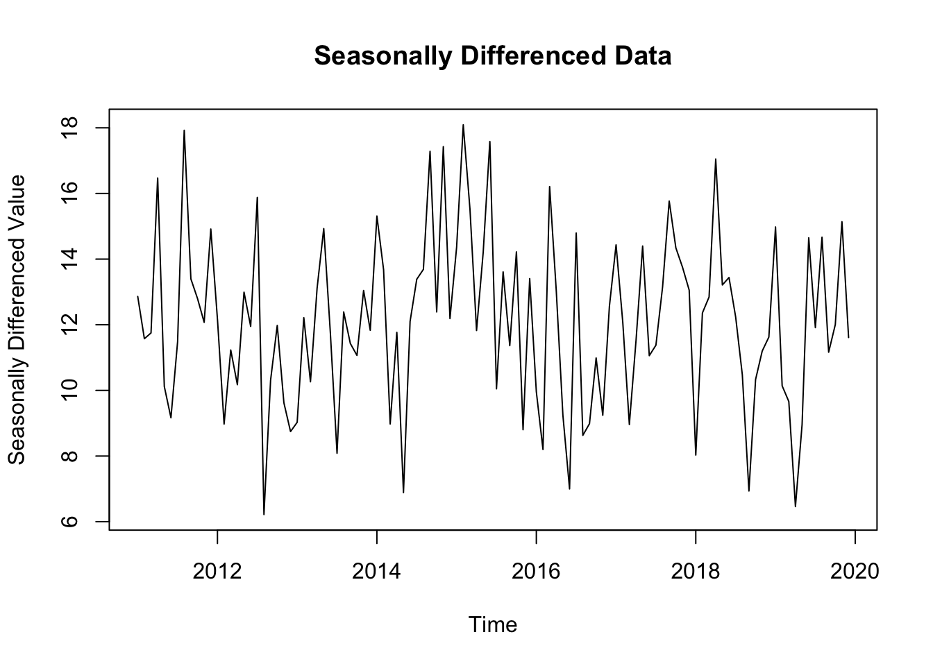
Additional note: seasonal differencing
If the time-series has a seasonal pattern, then seasonaldifferencing can be used. Here, the observation from the previous season is subtracted from the current observation.
Show code
s <-12# Example for monthly data with an annual cycle seasonal_diff_ts_data <-diff(ts_data, lag = s, differences =1)# Plot the seasonally differenced dataplot(seasonal_diff_ts_data, main="Seasonally Differenced Data", xlab="Time", ylab="Seasonally Differenced Value")
Step One: Remove the Time column from the dataframe.
Step Two: Convert the dataframe df to a time-series object. Use frequency = 12.
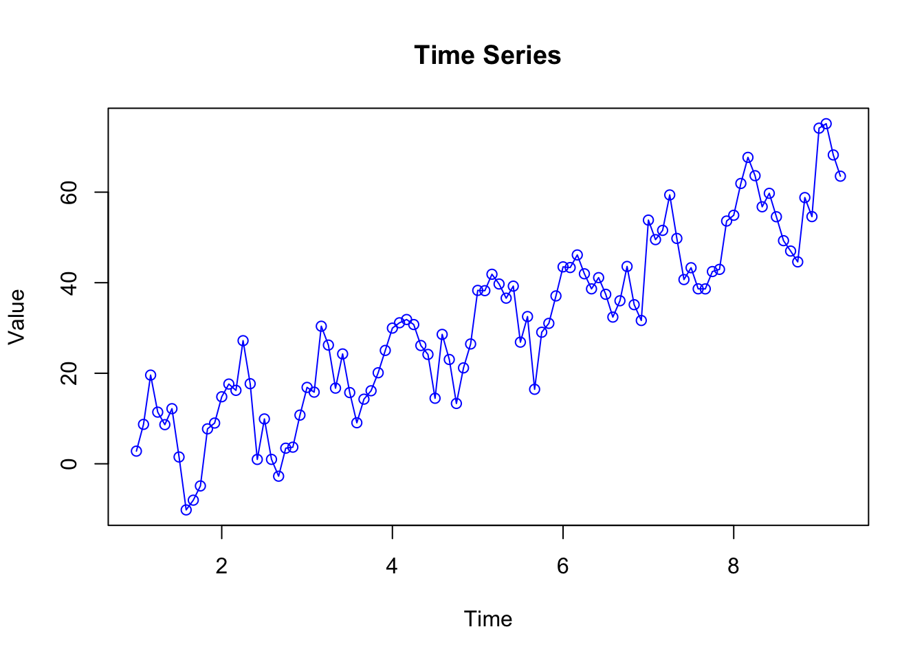
Step Three: Plot the time-series object.
Consider: does the time-series appear to be stationary or non-stationary?
Consider: does the time-series appear to have seasonality or not?
Step Four: Test the time-series object for stationarity using the ADF test.
Step Five: If required (based on the ADF), apply differencing to the time-series to address issues of stationarity.
Step Six: Test new time-series data for stationarity using the ADF.
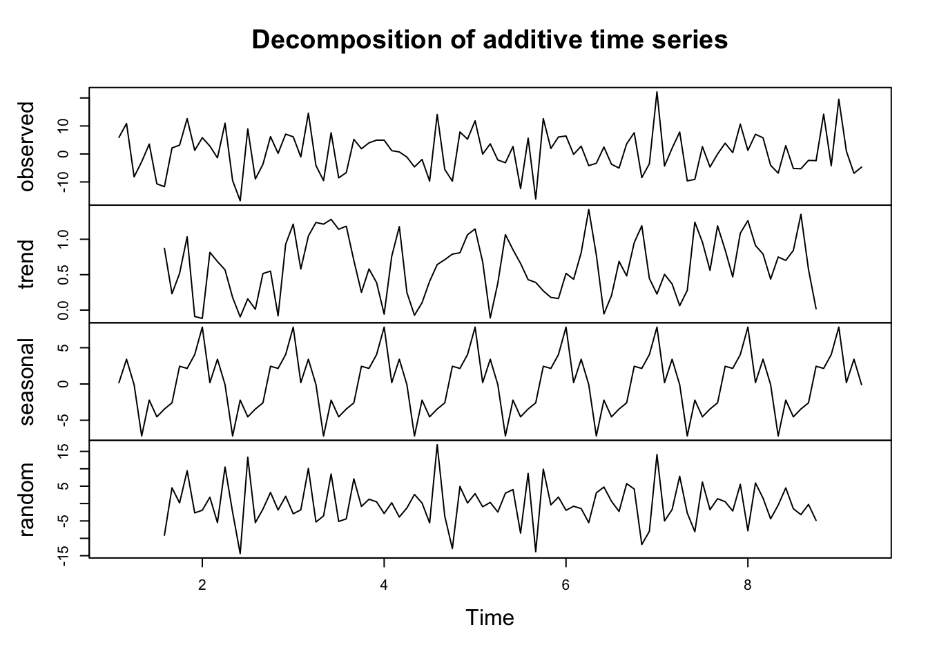
Step Seven: If stationarity has been achieved, decompose the new time-series data.
Consider: Is there a seasonal component to the data?
Show solution
# remove time columndf$Time <-NULL# convert dataframe to time-seriesdf_ts <-ts(df, frequency =12)# plot df_tsplot(df_ts, type ="o", col ="blue", main ="Time Series", xlab ="Time", ylab ="Value")
Show solution
# test for stationaritylibrary(urca)# Perform the Augmented Dickey-Fuller Testadf_test <-ur.df(df_ts, type ="drift", lags =1)# View the summary of the test, including critical valuessummary(adf_test)
###############################################
# Augmented Dickey-Fuller Test Unit Root Test #
###############################################

Test regression drift


Call:
lm(formula = z.diff ~ z.lag.1 + 1 + z.diff.lag)

Residuals:
     Min       1Q   Median       3Q      Max
-19.2588  -4.5697   0.7262   4.4189  21.1632

Coefficients:
            Estimate Std. Error t value Pr(>|t|)
(Intercept)  2.45705    1.43932   1.707   0.0911 .
z.lag.1     -0.05862    0.04004  -1.464   0.1464
z.diff.lag  -0.11745    0.10277  -1.143   0.2560
---
Signif. codes:  0 '***' 0.001 '**' 0.01 '*' 0.05 '.' 0.1 ' ' 1

Residual standard error: 7.41 on 95 degrees of freedom
Multiple R-squared:  0.04412,   Adjusted R-squared:  0.02399
F-statistic: 2.192 on 2 and 95 DF,  p-value: 0.1173


Value of test-statistic is: -1.4642 1.4572

Critical values for test statistics:
      1pct  5pct 10pct
tau2 -3.51 -2.89 -2.58
phi1  6.70  4.71  3.86
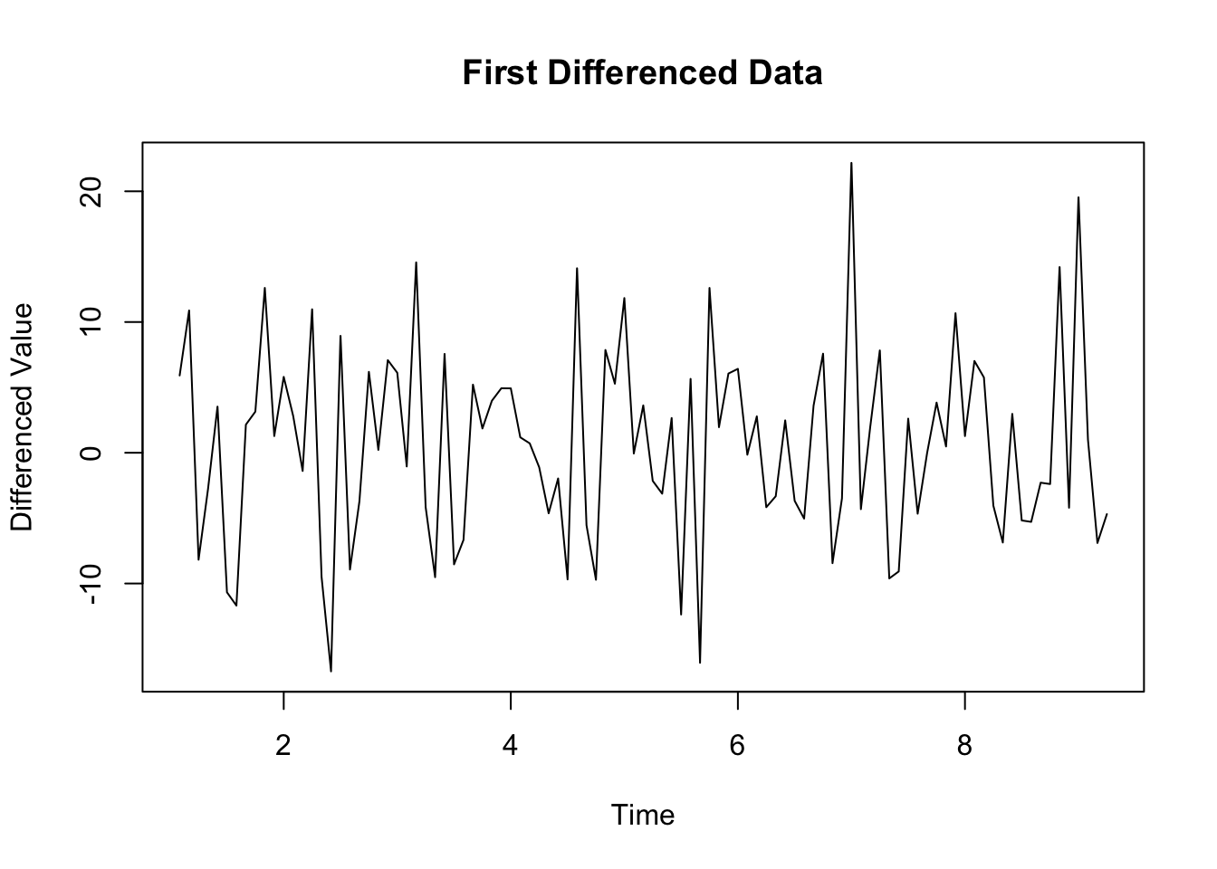
Show solution
# if needed, apply differencing and plot diff_df_ts <-diff(df_ts, differences =1) # create new object with differencing# Plot the differenced dataplot(diff_df_ts, main="First Differenced Data", xlab="Time", ylab="Differenced Value")
Show solution
# check new data with ADFadf_test <-ur.df(diff_df_ts, type ="drift", lags =1)# View the summary of the test, including critical valuessummary(adf_test)
###############################################
# Augmented Dickey-Fuller Test Unit Root Test #
###############################################

Test regression drift


Call:
lm(formula = z.diff ~ z.lag.1 + 1 + z.diff.lag)

Residuals:
     Min       1Q   Median       3Q      Max
-18.3992  -5.2393   0.5585   5.0858  20.5987

Coefficients:
            Estimate Std. Error t value Pr(>|t|)
(Intercept)  0.59128    0.76237   0.776    0.440
z.lag.1     -1.21538    0.15581  -7.800 8.36e-12 ***
z.diff.lag   0.04696    0.10249   0.458    0.648
---
Signif. codes:  0 '***' 0.001 '**' 0.01 '*' 0.05 '.' 0.1 ' ' 1

Residual standard error: 7.435 on 94 degrees of freedom
Multiple R-squared:  0.5851,    Adjusted R-squared:  0.5763
F-statistic: 66.29 on 2 and 94 DF,  p-value: < 2.2e-16


Value of test-statistic is: -7.8003 30.4705

Critical values for test statistics:
      1pct  5pct 10pct
tau2 -3.51 -2.89 -2.58
phi1  6.70  4.71  3.86
Show solution
# if stationarity has been achieved, decompose the time-series# Seasonal and Trend Decompositiondecomposed_data <-decompose(diff_df_ts)plot(decomposed_data)